Logrithmic Transformations
Examining Predictors of Wine Price
Investigating the Relationship
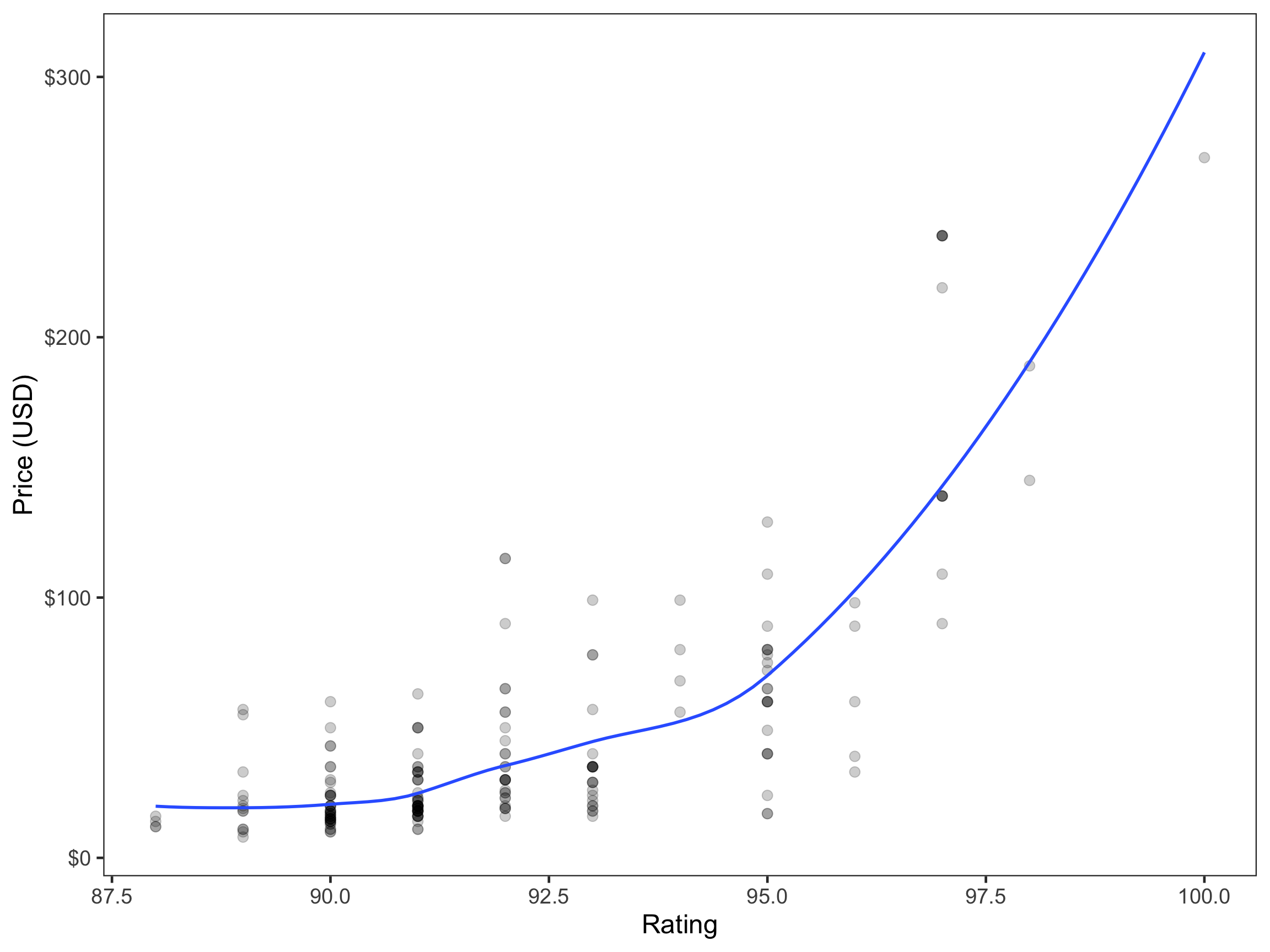
The literature has suggested that the price of wine is predictive of a wine’s rating which attempts to quantify a wine’s quality on a 100pt scale (Snipes & Taylor, 2014). Therefore, the relationship between wine rating and price was evaluated. The following scatter plot demonstrates this relationship for 200 wines made in seven geographic regions.
This figure shows a non-linear relationship between wine rating and price. In order to re-express the data to meet the linearity assumption of regression analyses, either the x (rating) or y-variable (price) must be transformed.
Creating Models
In accordance with the Rule of the Bulge, we elected to apply a downward power transformation to the y-variable by log-transforming wine price by the natural log. The natural log of wine price was then regressed on wine rating. The equation for this model is shown below:
\[ \begin{split} \mathrm{Model~1}: \hat{\mathrm{ln(Price_i)}} &= -19.06 + 0.25(\mathrm{Rating}_i) \end{split} \]
Two additional models were made to examine other possible predictors of price: one that only included the effects of whether or not a wine is made in California and another that included both wine rating and whether or not a wine is made in California:
\[ \begin{split} \mathrm{Model~2}: \hat{\mathrm{ln(Price_i)}} &= 3.46 + 0.015(\mathrm{California}_i) \\[1em] \mathrm{Model~3}: \hat{\mathrm{ln(Price_i)}} &= -19.48 + 0.25(\mathrm{Rating}_i) + 0.16(\mathrm{California}_i) \end{split} \]
Comparing Models
Using AICc and \({R}^2\) values to compare models, we determined that Model 3 was the most appropriate model for the data. The following table shows this comparison.
Table 1. Unstandardized Coefficients & Confidence Intervals for a Series of OLS Regresison Models Fitted to Estimate Variation in Price of Wines
=================================================================================
                                 Model 1           Model 2          Model 3
Rating                            0.245                              0.249
                              (0.216, 0.273)                     (0.220, 0.277)

Region = California (dummy)                         0.015            0.164
                                               (-0.207, 0.236)   (0.022, 0.305)

Intercept                        -19.059            3.456           -19.478
                            (-21.688, -16.429) (3.326, 3.586)  (-22.106, -16.851)

---------------------------------------------------------------------------------
AICc                              284.73           461.84            281.7
R2                                0.588            0.0001            0.598
Residual Std. Error               0.488             0.760            0.483
=================================================================================
Interpretting Model 3
In order to make a coherent, useful interpretation of Model 3, it is necessary to back-transform the model by exponentiating our equation by base-e. Rating = 1 and California = 1 were substituted into the equation to make sense of a one-unit change in each, and the equation was then simplified. The steps of this process are shown below.
\[ \begin{split} \hat{\mathrm{ln(Price_i)}} &= -19.48 + 0.25(\mathrm{Rating}_i) + 0.16(\mathrm{California}_i) \\[1em] \hat{\mathrm{Price_i}} &= e^{-19.48} \times e^{0.25(\mathrm{Rating}_i)} \times e^{0.16(\mathrm{California}_i)} \\[1em] \hat{\mathrm{Price_i}} &= e^{-19.48} \times e^{0.25(1)} \times e^{0.16(1)} \\[1em] \hat{\mathrm{Price_i}} &= (3.47 \times 10^{-9}) \times 1.28 \times 1.17 \end{split} \]
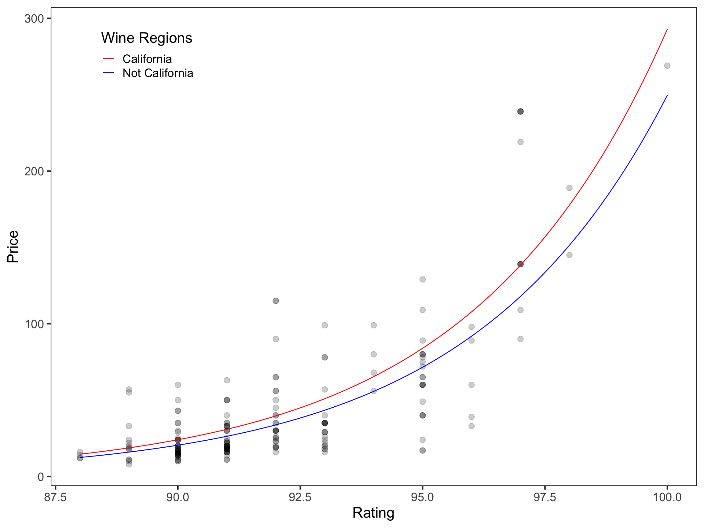
Drawing from this simplified model, we can conclude that on average, each one unit change in wine rating (i.e., 86 to 87) is associated with a 1.28-fold increase in the price of a wine. We can also conclude that being made in California (i.e., California = 1) is associated with a 1.17-fold increase in the price of a wine. Finally, the differential price between wines from California and those made in a different region to increase as rating increases due to interactions between rating and being made in California. The figure below demonstrates these findings.
